With increasing automation under high quality requirements the question about accuracies of the analysis plays an ever more important role. The more accurate the results of a computation are said to be, the more important it is to know, where they may be wrong.

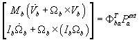
Basis of the calculations are often the following equations of motion proposed by Waszak et. al., which describe the dynamic response behaviour of a fully flexible aeroplane under appropriate and tested simplifications.

The first six degrees of freedom describe the nonlinear rigid body motion while the rest describes the flexible motion using a linear approach with a number of flexible modes. The equations are coupled in this formulation with external forces only.

Typically one key reason for deviations of computation versus reality are errors in the input data. During pre design these errors may be quite large, since many accurate measurements, e.g. wind tunnel tests, are still missing. In this situation it would be interesting to just roughly estimate the danger of an error in the results to get a feeling for the risk involved.

This can already well described estimating sensitivities

whereby usually only the effect of subranges of the input (e.g. uncertain masses/stiffnesses or external forces: Aerodynamics, Landing gear model) on subranges of the output (e.g. typically dimensioning loads) are of interest. This restriction allows a reduction of the problem to a few degrees of freedom only.

Sensitivities can efficiently be determined using automatic differentiation, which can be applied even to industrial large scale problems.

However, to get a better insight into the risk involved, stochastic methods may be helpful. Assuming distributions for incoming parameters, which itself can be an enormous difficulty, risk barriers can be defined on the outputs.

This can be achieved using the Fokker-Planck-Equation, which has the charming side effect of providing hard error bounds if solved with according methods.

Given an ordinary differential equation

an initial distribution of the probability density

is propagated through time according to

However, as simple as this equation looks, it becomes difficult to be solved in larger systems due to the “curse of dimensionality”. Particle methods as well as grid techniques are appropriate each with some simplifications each and topic of ongoing research.

For publications see [1].